Spawning Decay Analysis • DSMhabitat

library(DSMhabitat)

Objective

The objective of this analysis is to create flow-decay curves that will be applied to spawning habitat values at runtime in DSM models. The SRH2D model developed as part of the Sediment Study for the Upper Sacramento River serves as the starting point for these curves. Additional “scale-downs” are performed to reduce the magnitude of the curves in order to better match the observed relationship at each watershed where the analysis is applied. Each step in the analysis is detailed below.

SRH2D Flow-Sediment Transport Curves

Flow-to-sediment transport curves were obtained from the SRH2D model output. In total, there are 45 files, each representing a river mile. Each file contains 3 flow-to-sediment curves (in cubic meters per second) for three curve types: Parker, Wilcock, and Gaeuman. A sample output at river mile 283.330 is shown below.


files_to_read <- list.files(system.file("extdata", "spawning-decay", "SedimentRatingCurves", 
                                        package = "DSMhabitat", mustWork = TRUE),
                            pattern = ".txt", 
                            full.names = TRUE)

rating_curves_by_rm <- map_df(files_to_read, function(x) {
  river_mile <- str_match(basename(x), "[0-9]+\\.?[0-9]+")[,1]
  read_tsv(x, skip = 1, col_names = c("flow", "parker_qs", "wilcock_qs", "gaeuman_qs")) |> 
    mutate(river_mile = as.numeric(river_mile))
})

rating_curves_by_rm |> 
  filter(river_mile == 283.330) |> 
  knitr::kable()

flow	parker_qs	wilcock_qs	gaeuman_qs	river_mile
210	0.000071	0.000096	0.000246	283.33
500	0.004994	0.001350	0.003240	283.33
750	0.036029	0.005301	0.013065	283.33
1000	0.150990	0.016174	0.039437	283.33
1250	0.368879	0.036586	0.085184	283.33
1500	0.634368	0.064214	0.142707	283.33
2000	1.362871	0.149516	0.307467	283.33
2240	1.774680	0.202681	0.406075	283.33

All data was converted to cubic feet per second and two levels of summaries were performed. First, at each river mile, the minimum, average, and maximum values for transport were calculated across the three different curve types. Then, an average of transport was calculated for each combination of flow and minimum, mean, and maximum transport values across all the river miles. The code for the calculation is outlined below.

rating_curve <- rating_curves_by_rm |> 
  rename(flow_cms = flow) |> 
  pivot_longer(parker_qs:gaeuman_qs, names_to = "curve", values_to = "transport_m3_per_second") |> 
  mutate(
    flow_cfs = 35.315 * flow_cms,
    flow_cfd = flow_cfs * 86400, # cubic feet per day
    transport_ft3_per_second = 35.315 * transport_m3_per_second,
    transport_ft3_per_day = 86400 * transport_ft3_per_second # transport per day
  ) |> 
  group_by(flow_cfs, river_mile) |> # summary across 3 curve types 
  summarise(
    sed_ft3_per_second_min = min(transport_ft3_per_second), 
    sed_ft3_per_second_avg = mean(transport_ft3_per_second),
    sed_ft3_per_second_max = max(transport_ft3_per_second),    
    sed_ft3_per_day_min = min(transport_ft3_per_day), 
    sed_ft3_per_day_avg = mean(transport_ft3_per_day),
    sed_ft3_per_day_max = max(transport_ft3_per_day)
  ) |> 
  ungroup() |> 
  group_by(flow_cfs) |> # summary across all river miles
  summarise(
    sed_ft3_per_second_min = mean(sed_ft3_per_second_min), 
    sed_ft3_per_second_avg = mean(sed_ft3_per_second_avg),
    sed_ft3_per_second_max = mean(sed_ft3_per_second_max),
    sed_ft3_per_day_min = mean(sed_ft3_per_day_min), 
    sed_ft3_per_day_avg = mean(sed_ft3_per_day_avg),
    sed_ft3_per_day_max = mean(sed_ft3_per_day_max),
  ) |>
  ungroup() |> 
  mutate(flow_cfd = flow_cfs * 86400)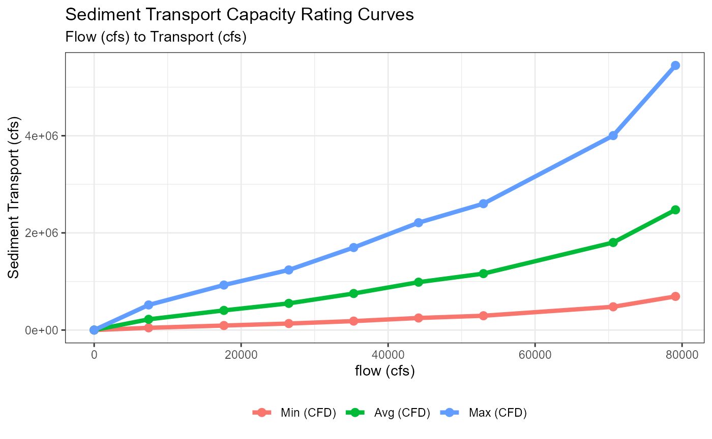

Curve Scale-downs

A series of scale-downs were performed next. The specific procedures for each scale-down are outlined in this section.

Gravel size based scaledown

The initial reduction in scale was based on a flow-to-gravel size movement curve, which, given the flow and size of gravel, calculates the proportion of gravel that is moving. This curve was obtained by digitizing a bar plot from the Gravel Study for the Upper Sacramento River. To align it with the flow-to-transport curves, we calculated the minimum, mean, and maximum values across the four reaches, and interpolated flows to match those in the flow-to-transport curves.

gravel_size_scaledown <- read_csv(system.file("extdata", "spawning-decay", "sediment-prop-move.csv", 
                                              package = "DSMhabitat", mustWork = TRUE))

gravel_size_to_prop_of_movement <- gravel_size_scaledown |> 
  mutate(
    flow_cfs = flow_m3s * 35.315,
    flow_cfday = flow_cfs * 86400) |> 
  group_by(flow_cfs) |> 
  summarise(
    min_fraction = min(fraction), 
    avg_fraction = mean(fraction),
    max_fraction = max(fraction)
  ) |> 
  bind_rows(
    tibble(flow_cfs = 0, min_fraction = 0, avg_fraction = 0, max_fraction = 0) # adds 0,0,0 case to match transport curves
  )

knitr::kable(gravel_size_to_prop_of_movement)

flow_cfs	min_fraction	avg_fraction	max_fraction
7416.15	0.0806018	0.0968323	0.1217712
17657.50	0.1941146	0.2733349	0.3368477
26486.25	0.3025297	0.4197242	0.4928835
35315.00	0.3830666	0.5127448	0.6088125
44143.75	0.4161074	0.5452193	0.6550242
52972.50	0.4367579	0.5705558	0.7044600
70630.00	0.4470831	0.5785127	0.7442235
79105.60	0.4288639	0.5421749	0.7603439
0.00	0.0000000	0.0000000	0.0000000

gravel_size_to_prop_of_movement |> 
  pivot_longer(names_to = "prop_type", values_to = "Proportion able to Move", -flow_cfs) |> 
  ggplot(aes(flow_cfs, `Proportion able to Move`, color = prop_type)) +  
  geom_line(size = 1.5) + 
  geom_point(size = 2.5)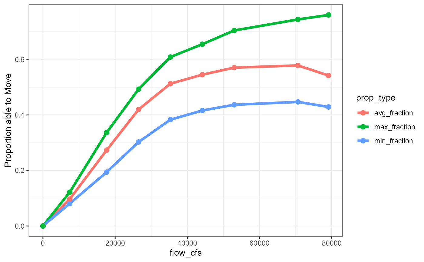

First Scaledown Curve Application

The method we use to generate these scaled-down curves is the approxfun function generator in R. The following outlines the process. Note that at this point we must choose between one of three (min, mean, max) curves to use as the input into approxfun.

# using the min

min_sfd_gravel_size_red <- approxfun(
  x = srh2d_upper_sac_rating_curves$flow_cfs, 
  y = srh2d_upper_sac_rating_curves$sed_ft3_per_day_min * 
    gravel_size_to_prop_of_movement$avg_fraction
)
avg_sfd_gravel_size_red <- approxfun(
  x = srh2d_upper_sac_rating_curves$flow_cfs, 
  y = srh2d_upper_sac_rating_curves$sed_ft3_per_day_avg * 
    gravel_size_to_prop_of_movement$avg_fraction
)
max_sfd_gravel_size_red <- approxfun(
  x = srh2d_upper_sac_rating_curves$flow_cfs, 
  y = srh2d_upper_sac_rating_curves$sed_ft3_per_day_max * 
    gravel_size_to_prop_of_movement$avg_fraction
)

We can recalculate the transport curves with this scaledown by apply our generated functions above.

min_sfd_with_gravel_scale <- tibble(
  flow_cfs = srh2d_upper_sac_rating_curves$flow_cfs, 
  transport_cfd = min_sfd_gravel_size_red(flow_cfs), 
  type = "min"
)

avg_sfd_with_gravel_scale <- tibble(
  flow_cfs = srh2d_upper_sac_rating_curves$flow_cfs, 
  transport_cfd = avg_sfd_gravel_size_red(flow_cfs), 
  type = "mean"
)

max_sfd_with_gravel_scale <- tibble(
  flow_cfs = srh2d_upper_sac_rating_curves$flow_cfs, 
  transport_cfd = max_sfd_gravel_size_red(flow_cfs), 
  type = "max"
)

transport_scaled_by_gravel <- bind_rows(
  min_sfd_with_gravel_scale, 
  avg_sfd_with_gravel_scale, 
  max_sfd_with_gravel_scale
)


transport_scaled_by_gravel |> 
  ggplot(aes(flow_cfs, transport_cfd, color=type)) + geom_line(size = 1.5) + 
  geom_point(size = 2.5)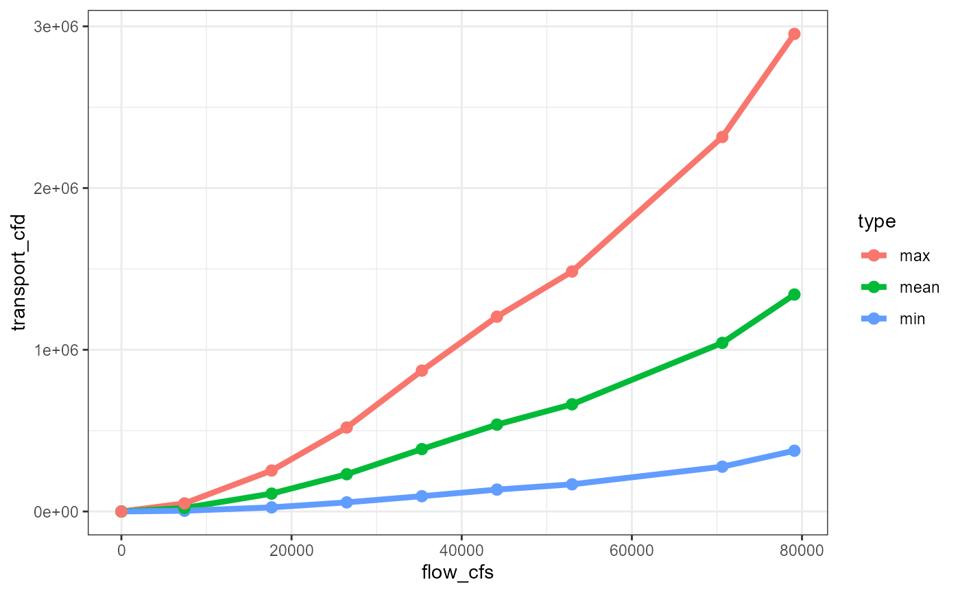

Storm Observed based Scaledown

The next scale-down is based on observed sediment transport and Market Bridge within the Upper Sacramento River. The approach is to develop a scale-down factor that allows the curves to match this observed event. The setup is simple: we start with a known amount of gravel and a known date at which the gravel was moved away. We create a function out of this process and feed it into an optimization process that finds the scale-down value that best matches the event.

kwk_usgs <- read_rds(system.file("extdata", "spawning-decay", "kwk-flows-1980-2022.rds", 
                                 package = "DSMhabitat", mustWork = TRUE))

objective_func <- function(threshold) {
  
  # scale down the tranport curves to just the d50mm threshold of movement
  scaled_sed_transport <- srh2d_upper_sac_rating_curves$sed_ft3_per_day_min * 
    gravel_size_to_prop_of_movement$avg_fraction
  
  # create an approxfun given a threshold of movement (this value will be searched by the optim function)
  calib_sed_curve <- approxfun(srh2d_upper_sac_rating_curves$flow_cfs, 
                               scaled_sed_transport * 
                                 rep(threshold, # <----- this value is searched 
                                     length(srh2d_upper_sac_rating_curves$flow_cfs)))
  
  # convert square meters to cubic feet, assume 2ft depth
  starting_volume <- (254690.3 * 10.764) * 2
  
  calib_kwk_sed_transport <- tibble(
    date = kwk_usgs$Date, 
    flow = kwk_usgs$Flow, 
    sediment_transport_f3_day = calib_sed_curve(flow)
  ) |> 
    mutate(sediment_transport_f3_day = ifelse(is.na(sediment_transport_f3_day), 0, sediment_transport_f3_day))
  
  
  calib_kwk_sed_transport_sim <- calib_kwk_sed_transport |> 
    filter(date >= "2015-01-01", date <= "2017-04-01") |> 
    mutate(sediment_transport_f3_day_accum = cumsum(sediment_transport_f3_day),
           current_vol = starting_volume - sediment_transport_f3_day_accum)
  
  # get the last value for volume
  last_volume <- calib_kwk_sed_transport_sim |> tail(1) |> pull(current_vol)
  
  # return absolute distance to zero
  return(abs(last_volume - 0))
}


# We want to optimize the function by the threshold value that results
# in the volumne nearest zero.
result <- optimise(objective_func, interval = c(0, 1), maximum = FALSE)

The optimise function returns: Scale-down value: 0.5099701, which gets us within 177.844 cubic feet of zero. We can evaluate this fit by plotting both the flow and volume decay on the same axis.

sac_river_observation_scaledown <- result$minimum

# create a new curve with this scaledown applied
flow_cfs_to_sed_cfd_calibrated <- approxfun(
  x = srh2d_upper_sac_rating_curves$flow_cfs, 
  y = srh2d_upper_sac_rating_curves$sed_ft3_per_day_min * 
    gravel_size_to_prop_of_movement$avg_fraction * 
    rep(sac_river_observation_scaledown, 
        length(srh2d_upper_sac_rating_curves$flow_cfs))
)

calibrated_kwk_sed_transport <- tibble(
  date = kwk_usgs$Date, 
  flow = kwk_usgs$Flow, 
  sediment_transport_f3_day = flow_cfs_to_sed_cfd_calibrated(flow)
) |> 
  mutate(sediment_transport_f3_day = ifelse(is.na(sediment_transport_f3_day), 0, sediment_transport_f3_day))


starting_volume <- (254690.3 * 10.764) * 2

kwk_sed_transport_sim <- calibrated_kwk_sed_transport |> 
  filter(date >= "2015-01-01", date <= "2017-04-01") |> 
  mutate(sediment_transport_f3_day = ifelse(is.na(sediment_transport_f3_day), 0, sediment_transport_f3_day), 
         sediment_transport_f3_day_accum = cumsum(sediment_transport_f3_day),
         start_vol = starting_volume,
         current_vol = start_vol - sediment_transport_f3_day_accum)

p1 <- kwk_sed_transport_sim |> 
  ggplot() + 
  geom_line(aes(date, current_vol)) + 
  labs(x = "", y = "Spawning Habitat Vol. (cubic feet)") + 
  theme_bw()

p2 <- kwk_usgs |> 
  filter(Date >= "2015-01-01", Date <= "2017-04-01") |> ggplot(aes(Date, Flow)) + geom_line() + 
  theme_bw()

# plot to confirm scaledown did the right thing
grid.arrange(p2, p1, nrow = 2)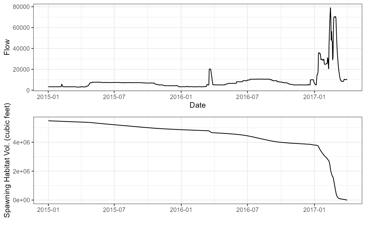

Second update to the transport curves

At this point, we can apply both scale-downs (gravel size and observed) to update our current transport curves. To do this, we simply apply both scale-downs in the function generation call to approxfun.

min_sfd_gravel_obs <- approxfun(
  x = srh2d_upper_sac_rating_curves$flow_cfs, 
  y = srh2d_upper_sac_rating_curves$sed_ft3_per_day_min * 
    gravel_size_to_prop_of_movement$avg_fraction * result$minimum
)

avg_sfd_gravel_obs <- approxfun(
  x = srh2d_upper_sac_rating_curves$flow_cfs, 
  y = srh2d_upper_sac_rating_curves$sed_ft3_per_day_avg * 
    gravel_size_to_prop_of_movement$avg_fraction * result$minimum
)

max_sfd_gravel_obs <- approxfun(
  x = srh2d_upper_sac_rating_curves$flow_cfs, 
  y = srh2d_upper_sac_rating_curves$sed_ft3_per_day_max * 
    gravel_size_to_prop_of_movement$avg_fraction * result$minimum
)

min_sfd_with_gravel_obs <- tibble(
  flow_cfs = srh2d_upper_sac_rating_curves$flow_cfs, 
  transport_cfd = min_sfd_gravel_obs(flow_cfs), 
  type = "min"
)

avg_sfd_with_gravel_obs <- tibble(
  flow_cfs = srh2d_upper_sac_rating_curves$flow_cfs, 
  transport_cfd = avg_sfd_gravel_obs(flow_cfs), 
  type = "mean"
)

max_sfd_with_gravel_obs <- tibble(
  flow_cfs = srh2d_upper_sac_rating_curves$flow_cfs, 
  transport_cfd = max_sfd_gravel_obs(flow_cfs), 
  type = "max"
)

transport_scaled_by_gravel_obs <- bind_rows(
  min_sfd_with_gravel_obs, 
  avg_sfd_with_gravel_obs, 
  max_sfd_with_gravel_obs
)


transport_scaled_by_gravel_obs |> 
  ggplot(aes(flow_cfs, transport_cfd, color=type)) + geom_line(size = 1.5) + 
  geom_point(size = 2.5) + 
  scale_y_continuous(labels = scales::comma)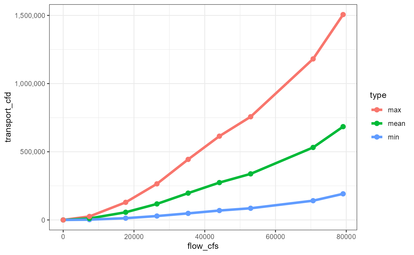

Experts based scale-down

The last series of scale-downs were developed with the help of John Hannon and Chris Hammersmark, both of whom are recognized as experts in the hydrology of the Upper Sacramento River. We evaluated the existing scale-downs and found that it was necessary to implement an additional set of reductions to account for gravel deposition This analysis involved the addition of augmentations, which will be explained in more detail in the following section.

Augmentation Data

To correctly evaluate the scale-downs, it is important to examine the augmentations that were performed in the Upper Sacramento River DSM watershed. We collected augmentations from John Hannon and augmentations listed in the Stillwater report dating back to 1978, and consolidated the data into total acres per year. A 2-foot depth was assumed in order to convert the information from tons.

# combine both John Hannon's data and augmentations from Stillwater report
sac_augmentation_totals <-
  upper_sac_augmentations |> 
  group_by(date) |> 
  summarise(tons = sum(tons)) |> 
  filter(!is.na(date)) |> 
  mutate(
    date = as_date(paste0(date, "-01-31")),
    cubic_yard = tons / 1.5, 
    cubic_feet = cubic_yard * 27,
    sq_feet = cubic_feet / 2, 
    acres = sq_feet / 43560,
    source = "H"
  ) |> 
  select(date, acres, source) |>  
  bind_rows(stillwater_sac_augmentations) |> 
  arrange(date) |> 
  filter(!is.na(acres))


gt(sac_augmentation_totals |> transmute(Year = format(date, "%Y"), Acres = round(acres, 2))) |> 
  tab_header(title = "Compiled Upper Sacramento Augmentations (1978-2022)") |> 
  tab_footnote(footnote = "data was converted from tons to acres, assuming a 2ft depth")

Year	Acres
Compiled Upper Sacramento Augmentations (1978-2022)
1978	1.43
1979	2.70
1988	4.96
1989	2.48
1990	30.97
1997	6.40
1998	4.75
1999	5.17
2000	6.61
2002	3.10
2003	1.82
2004	1.76
2005	1.49
2006	1.24
2007	1.24
2008	1.71
2009	2.05
2010	1.14
2011	1.03
2012	3.10
2013	2.89
2014	0.00
2015	0.00
2016	6.61
2017	2.89
2018	0.00
2019	6.61
2022	4.13
data was converted from tons to acres, assuming a 2ft depth

sac_augmentation_totals |> 
  mutate(year = year(date)) |> 
  ggplot(aes(year, acres)) + geom_col() + 
  scale_x_continuous(breaks = seq(1978, 2022, by = 2)) + 
  ggplot2::theme(axis.text.x = element_text(angle = 90)) + 
  labs(x = "")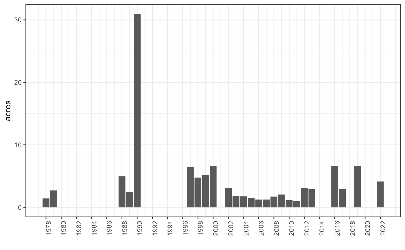

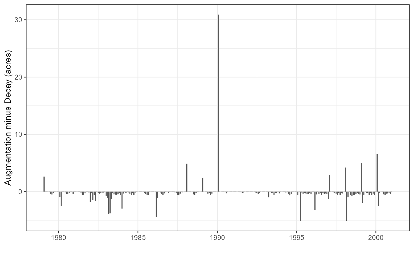
Augmentation and Decay

In this section, we utilize the decay curve that we have constructed up to this point, along with DSM flows, to predict decay. The resulting time series is then analyzed, and additional scale-downs are determined based on expert opinions. Discussions have indicated that, taking augmentations and decays into consideration, it is estimated that there will be approximately 2 acres of decay per year on average. As a result, an additional scale-down factor of .19 will be applied as the final scale-down.

# Use DSM flows to determine decay
upper_sac_flows_dsm <- DSMflow::flows_cfs$biop_2008_2009 |>
  filter(year(date) >= 1979, year(date) <= 2000) |>
  select(date, flow = `Upper Sacramento River`)

# combine decay and calculate acres
upper_sac_decay <- tibble(
  date = upper_sac_flows_dsm$date,
  flow = upper_sac_flows_dsm$flow,
  decay_cfd = ifelse(is.na(
    (x <- min_sfd_gravel_obs(flow))),
    0, x
  ),
  decay_cfm = decay_cfd * days_in_month(month(date)),
  decay_sqm = decay_cfm / 2,
  decay_acres_month = decay_sqm / 43560
)

# scale-down to achieve annual average decay of 2 acres
domain_expert_additional_scaledown <- .19

decays <- upper_sac_decay |> select(date, decay_acres_month, flow) |>
  mutate(scaled_decay = decay_acres_month * domain_expert_additional_scaledown)

augmentations <- sac_augmentation_totals |> select(date, aug_acres=acres)

decays_and_augs <- decays |>
  left_join(sac_augmentation_totals, by=c("date"="date")) |>
  mutate(acres = ifelse(is.na(acres), 0, acres),
         aug_minus_decay = acres - decay_acres_month,
         aug_minus_decay_scaled = acres - scaled_decay,
         month = month(date),
         year = year(date))

decays_and_augs |>
  group_by(year) |>
  summarise(
    avg_diff = mean(aug_minus_decay_scaled),
    sum_loss = sum(aug_minus_decay_scaled)
  ) |>
  pull(sum_loss) |>
  mean()
#> [1] -1.967822


decays_and_augs |> 
  ggplot(aes(date, aug_minus_decay_scaled)) + geom_col() +
  labs(x = "", y = "Augmentation minus Decay (acres)")